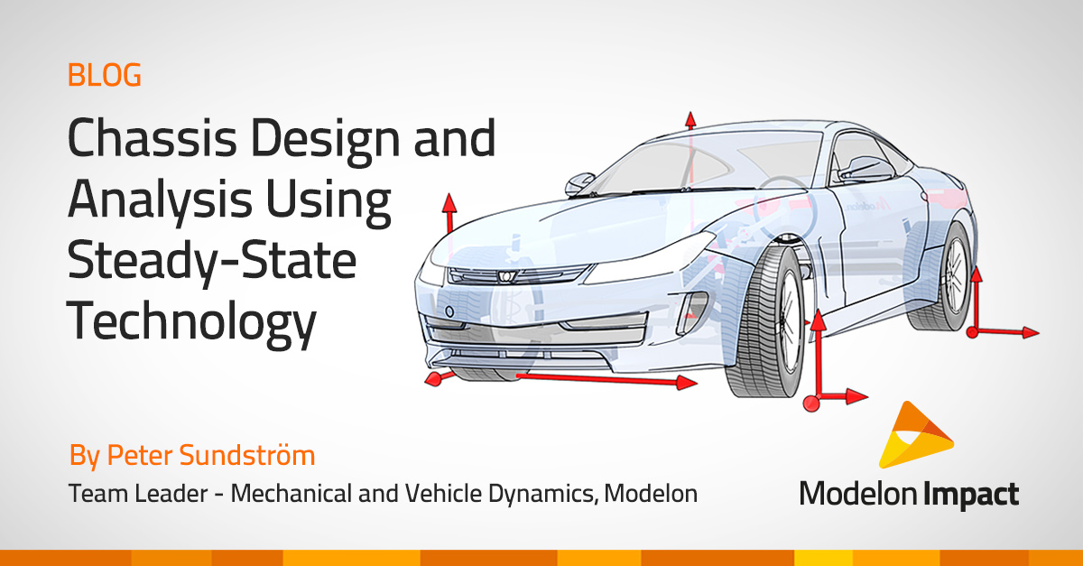
Multi-body Vehicle Dynamics: Chassis Design and Analysis Using Steady-State Technology
This blog post focuses on the modeling and simulation of chassis in Modelon Impact. Modelon Impact’s steady-state solver and multi-execution capabilities make it possible to achieve steady-state analysis with speed and precision for multi-body vehicle dynamics.
Part 1 of this blog series, Efficient Suspension Design in Modelon Impact, focuses on the design and analysis of the suspension system. This is now possible with the Modelon 2022.1 Release.
Chassis Modeling and Design using Modelon’s Vehicle Dynamics Library

In this analysis, we will use a simple, polynomial-based vehicle model to directly define the high-level characteristics of the vehicle and its suspensions. We can use this model to get our overall chassis behavior in place, which naturally generates targets for suspension design. Once the suspension is designed, we can run the same analysis with the multibody suspension to verify
our targets.
Quasi-Static Analysis
As a first step, the steady-state behavior of the vehicle needs to be understood. As a car is taken through different speeds and levels of lateral acceleration, we can analyze how the forces are distributed over the two axles, how the roll moment distribution affects lateral load transfer, and the fundamental handling characteristics of the vehicle.
To put the chassis into the desired state, quasi-static analysis needs to be applied and is conveniently available in Modelon’s Vehicle Dynamics Library. The quasi-static analysis uses a robot that forces the chassis into the desired state which, without changing the driver inputs, would lead to forces and torques applied to the chassis. The steady-state solution gives us the inputs needed to maintain the desired state without any external forces applied. With Modelon Impact, we can directly solve for the steady-state case.
Handling Diagram
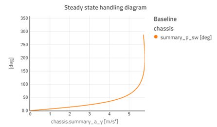
To evaluate the steady-state behavior of our chassis, we will look at the handling diagram. The handling diagram shows the required steering wheel angle to maintain a given level of lateral acceleration. This will give us the understeer gradient as well as the maximum lateral acceleration we can achieve. A positive understeer gradient, meaning there will be more steering angle required as we increase the lateral acceleration, car is “understeered.” Generally, this is desirable for a passenger car because it is more stable. For sports cars or racing cars, a lower understeer gradient will give a more responsive car at the expense of stability.
With the steady-state solver in Modelon Impact and appropriate experiment templates, we can set up a pure steady-state solution to get the handling diagram. This eliminates any dynamic effects from stiffnesses in the suspension and the need to have controller components maintaining either the constant speed or the constant corner radius. This is because both are solved in the steady-state solution.
Figure 1 shows the handling diagram for our example chassis model at 100km/h. All subsequent diagrams are for the same speed.
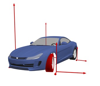
For each result point, we have access to the complete output from the chassis model so we can look at all the variables at every point. In addition to this, the visualization capabilities recently introduced in Modelon Impact allow us to look at the visualization of the vehicle as it goes through the test, as seen in Figure 2.
With the baseline above, we can start looking at varying parameter sweeps to see how they affect our handling diagram. First, we will look at what happens when we adjust the longitudinal position of the center of gravity. Figure 3 shows the handling diagram sweep as longitudinal position of the sprung mass center of gravity is swept from -1.0—1.5m relative to the front axle in 20 steps. To give an idea of the performance, this sweep calculates 100 steady-state points for each of the 20 cases and the whole analysis completes in around 15 seconds for the polynomial model.
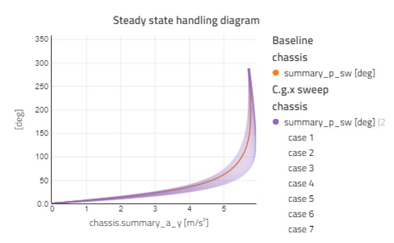
This shows the expected result where moving the c.g. further forward in the car makes the car more stable, but also gets a lower peak lateral acceleration. The c.g. further rear gives us a more responsive car with a higher peak lateral acceleration.
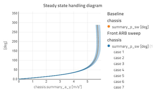
Next, we will look at the antiroll bar stiffness. Figure 4 shows a sweep of the front antiroll bar stiffness from 150 to 300 Nm/rad in 15 steps. This has the biggest effect for higher lateral accelerations where the roll moment is higher. A stiffer front anti-roll bar takes up more of the overall roll moment at the front axle which reduces the grip available for steering giving a lower peak lateral acceleration.
The quasi-static robot component we use to apply forces and torques to the chassis allows us to set how the drive and brake torques are distributed between the axles. This lets us look at brake bias and different variants of drive torque distribution. Figure 5 shows how the handling diagram at a deceleration of -3 m/s2 changes as we vary brake bias from 50% to 100% at the front axle.
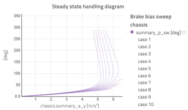
In Figure 5, there are only the 6 cases with the most braking at the front which aids in finding a solution for the complete range of steer input. This corresponds to a front brake bias of 82% and up.
Finally, we will look at suspension kinematics. In Figure 6, we run a sweep of the bump steer ratio (toe angle vs wheel travel) from -11.5 to 11.5 °/m at the front suspension with the front brake bias of 82% as selected above.
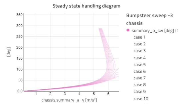
Figure 6 shows that suspension kinematics have a big impact on vehicle stability. This is a way to find the overall kinematic targets of your suspension and match them with other properties like mass distribution, roll moment distribution, and brake/drive torque distribution.
Dynamic Response of A Vehicle
Once we have the steady-state handling characteristics we can look at the dynamic response of the vehicle. This includes analyzing the frequency response and running a step steer experiment.
Frequency Response
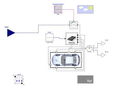
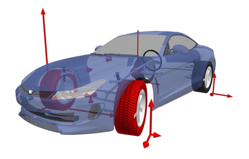
The frequency response analysis shows how the vehicle will respond to steering inputs of different frequencies. This is done in Modelon Impact by letting the vehicle stabilize at the desired speed then linearizing the model with steering as input. The model is shown in Figure 7.
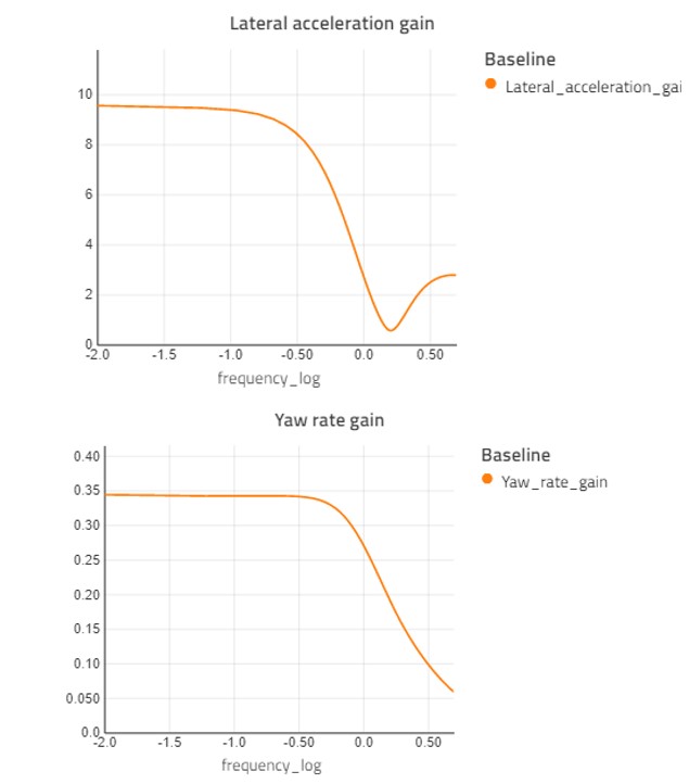
By running frequency analysis, we see what amplification results from a steering angle input of a particular frequency, to yaw rate and lateral acceleration, as shown in Figure 8.
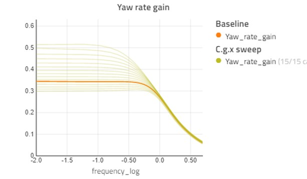
Like the steady-state analysis, we can run parameter sweeps to investigate how the frequency response changes. Figure 9 shows the for the same c.g. position sweep we did previously, the longitudinal c.g. position varying from -1m to -1.5m.
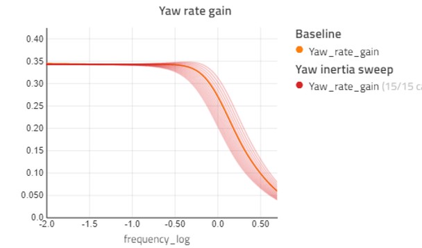
Another thing to study is the effect of varying yaw inertia of the vehicle. Figure 10 shows the yaw rate gain when varying the yaw inertia from 1500 to 3000 kgm2. This has very little effect in the lower frequencies, meaning it would not have any noticeable effect in the steady-state handling diagram. In the higher frequencies, however, it has a big impact on the response of the vehicle.
Step Steer
A simple test to conduct is a step steer. At a given speed, we apply a step in the steering wheel angle to view the different motion states of the vehicle are affected. This gives us insight into the responsiveness of the vehicle. While it is entirely possible in simulation, it is generally not feasible to apply a true step signal on the steering input in the physical car, so usually, some kind of ramp is used for the step input.
Figure 11 shows the results of a step steer of 0.5 radians at 100km/h. This shows how the lateral acceleration responds first to the step input. Then, as the vehicle starts to generate sideslip the yaw rate starts building up. The result is the steady-state response as done in the steady-state handling diagram, also seen as the steady-state gain in the frequency response.
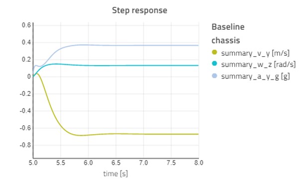
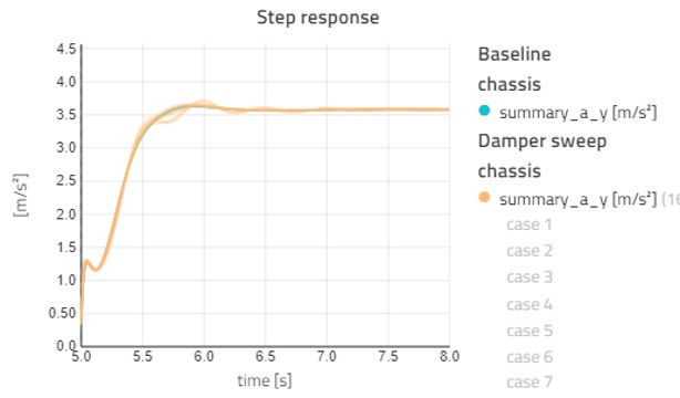
Figure 12 shows the effects of changing the damper settings of the vehicle. Figure 12 shows the lateral acceleration response to a step steer as we vary the front and rear dampers from 1000 to 8000 Ns/m in 4 steps each. When sweeping multiple parameters, Modelon Impact will run all combinations –ending up with 16 cases in total.
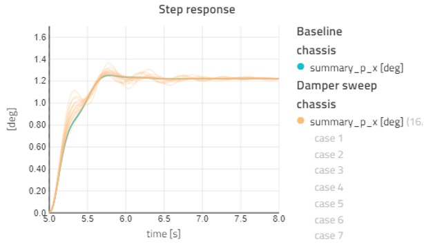
The effects of varying damper values are more obvious when looking at the roll angle response. Figure 13 shows the roll angle response to the same damper sweep as shown above.
Closing the Loop with Vehicle Dynamics Library in Modelon Impact
In the analyses above, we utilized the simple chassis model to find the right overall characteristics and targets for suspension design. When suspension design is started, we can then use multi-body suspensions in the same analyses to verify that we meet our chassis-level targets.
With Modelon’s Vehicle Dynamics Library, coupled with Modelon Impact, all different fidelity levels of chassis models fit into the same experiment templates. So, you can use simple models to set up your overall targets and characteristics, then maintain those same analyses as you further refine your design all the way to production.
Conclusion
Modelon’s Vehicle Dynamics Library, coupled in Modelon Impact, is even more powerful with the addition of steady-state simulations and multi-execution. We aim to provide an easy-to-use toolchain where users can get answers quickly. Modelon’s Vehicle Dynamics Library covers a wide range of use cases from suspension and chassis design to real-time deployment and driver-in-the-loop simulators. Modelon can help, so reach out!