Spline-Based Table Look-Up Media Creator: Seamlessly Integrated Into Modelon Impact
This blog will cover the Spline-Based Table Look-Up (SBTL) Media Creator that has been seamlessly integrated into Modelon Impact. Below we review the general workflow along with how to access and use the tool, including a step-by-step example that proves the benefit of speed – 4 times faster to simulate.
What is Spline-Based Table Look-up?
SBTL is a modeling method used for accelerating simulations without compromising accuracy. The SBTL method is integrated in Modelon’s Air Conditioning Library (ACL) or Vapor Cycle Library (VCL) to create new computationally efficient implementations of existing working fluids. SBTL offers a significant improvement in execution time, in comparison to an equivalent Helmholtz-implemented fluid, while maintaining the same physical accuracy.
The number of SBTL implemented fluids currently provided in ACL and VCL is expanding. We have had many customers request other fluids in addition to the already existing ones in the library.
What is the Spline-Based Table Look-up Media Creator?
To enable our library users to create their own spline-based media, an SBTL media creation tool has been developed in Python 3.7 and released together with Modelon Impact (note that the creation tool is available on all platforms that support ACL and VCL though this blog focuses on the integration with Modelon Impact). The tool enables the user to automatically create SBTL two-phase fluid models in Modelica with very little input required. The generated fluid models can then be loaded in Modelon Impact and further used in system simulations. The SBTL Media Creator requires either REFPROP 10.0 or CoolProp to generate all thermodynamic data necessary to create a two-phase fluid model in Modelica.
The SBTL Media Creator is delivered to our customers together with the Modelon Base Library (MBL). In the Modelon Impact installation directory, the SBTL Media Creator is found in the Modelon 3.5 folder in the modelica-dist directory. Included files in the SBTL media creator are displayed in Figure 1.
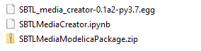
The .egg-file contains all the compiled Python code needed in the generation of a two-phase SBTL fluid model. A Jupyter notebook, SBTLMediaCreator.ipynb, is delivered as a user-friendly interface which guides the user through all the steps required to generate the data and Modelica files for a specific two-phase fluid. SBTLMediaModelicaPackage.zip is a compressed file containing the Modelica class templates that are needed in the code auto-creation step.
How does the Spline-Based Table Look-Up Media Creator Work?
A simplified workflow of the SBTL Media Creator is shown in Figure 2 below. In the first step, thermodynamic data, i.e. solutions to equations of state and transport properties, are generated for a user-specified fluid. All the data is generated using either Coolprop or REFPROP 10 as part of the backend. When all the thermodynamic properties have been extracted, additional data files and spline coefficients, that are necessary to fully implement the SBTL medium are created.
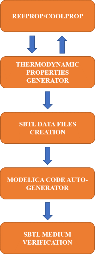
Once the required data files are successfully created, the tool will in the next step automatically generate all Modelica code necessary to utilize the SBTL media in system simulations. In the last step, the created SBTL medium is verified by simulating a small model that calls all the relevant medium functions. The simulation output will be compared to the values from Coolprop/REFPROP. The user can then examine the deviations in auto-generated performance plots and decide if the accuracy (depending on the user’s input to the tool) is sufficient. The verification step will also reveal if there are any potential numerical convergence issues with the generated SBTL medium.
Using Spline-Based Table Look-Up in Modelon Impact
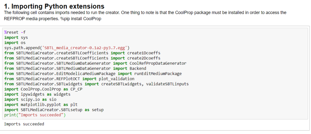
Step 1) The Jupyter notebook works as an interface between the user and the SBTL media creator. Once the Jupyter notebook is opened, the user will see a mix of code cells and detailed documentation on what the code does, as shown in Figure 3. The notebook code cells must be executed top-down.
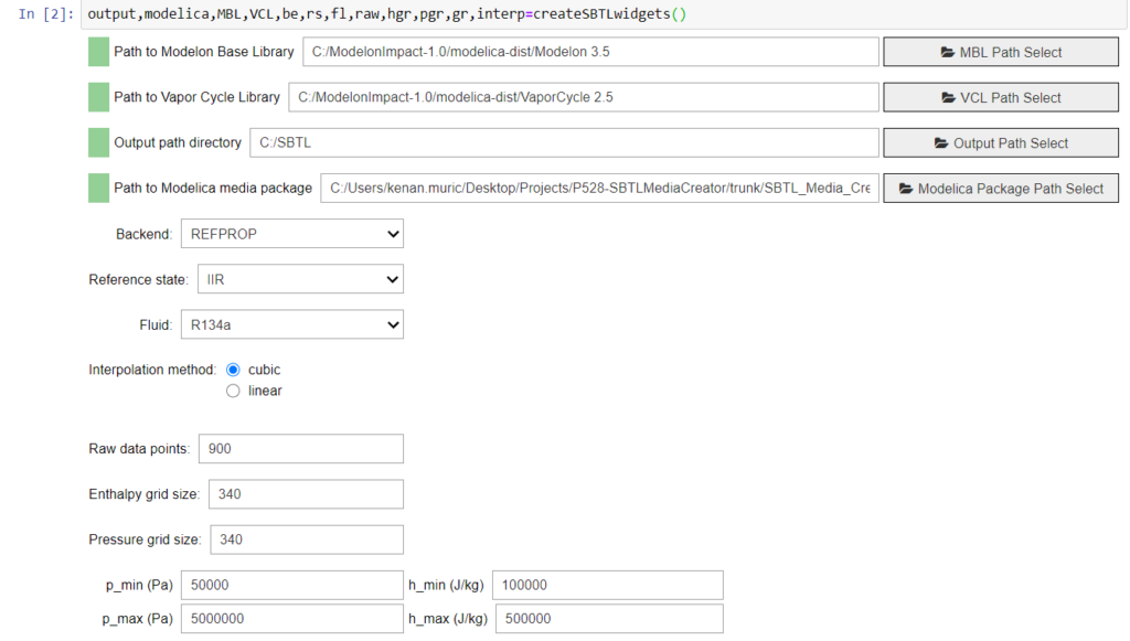
Step 2) Next, the user will reach the cell where all required input to the SBTL Media Creator needs to be entered, as seen in Figure 4.
Step 3) Verification plots for the created R134a SBTL medium are displayed in Figure 5 for density and entropy. The red line is the two-phase boundary for R134a. As can be seen, the accuracy is very high!

Step 4) We can now load the created SBTL medium into Modelon Impact by importing the Modelica package as a compressed file, as follows below.
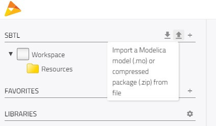
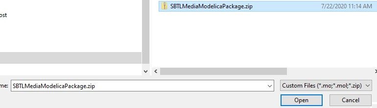
The SBTLMediaModelicaPackage.zip below contains the Modelica code generated by the SBTL media creator. We must compress the folder ourselves to load it into Modelon Impact.
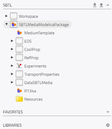
If successfully loaded, the workspace will now contain the SBTLMediaModelicaPackage.
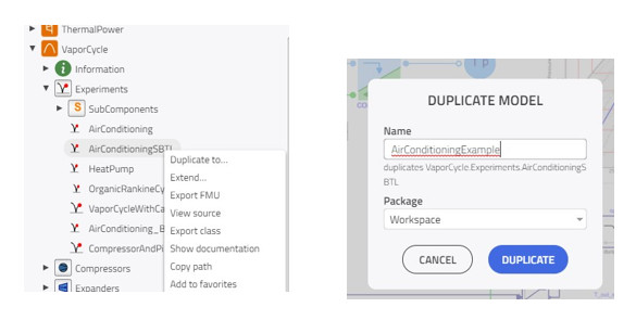
Step 5) Now we will duplicate the example VaporCycle.Experiments.AirConditioningSBTL from the Modelon Impact libraries to the workspace and name it AirConditioningExample.
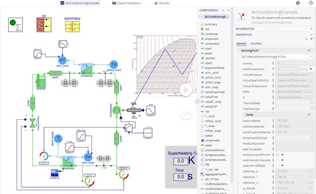
Step 6) We can now edit the working fluid in AirConditioningExample to the created R134a SBTL medium by editing the highlighted field in the parameter list seen below.
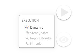
Step 7) Now we can run a dynamic simulation of the air-conditioning system by pressing the button seen below (execution type should be ‘Dynamic’).
Step 8) When the system simulation has completed, the results can be analyzed directly in Modelon Impact.
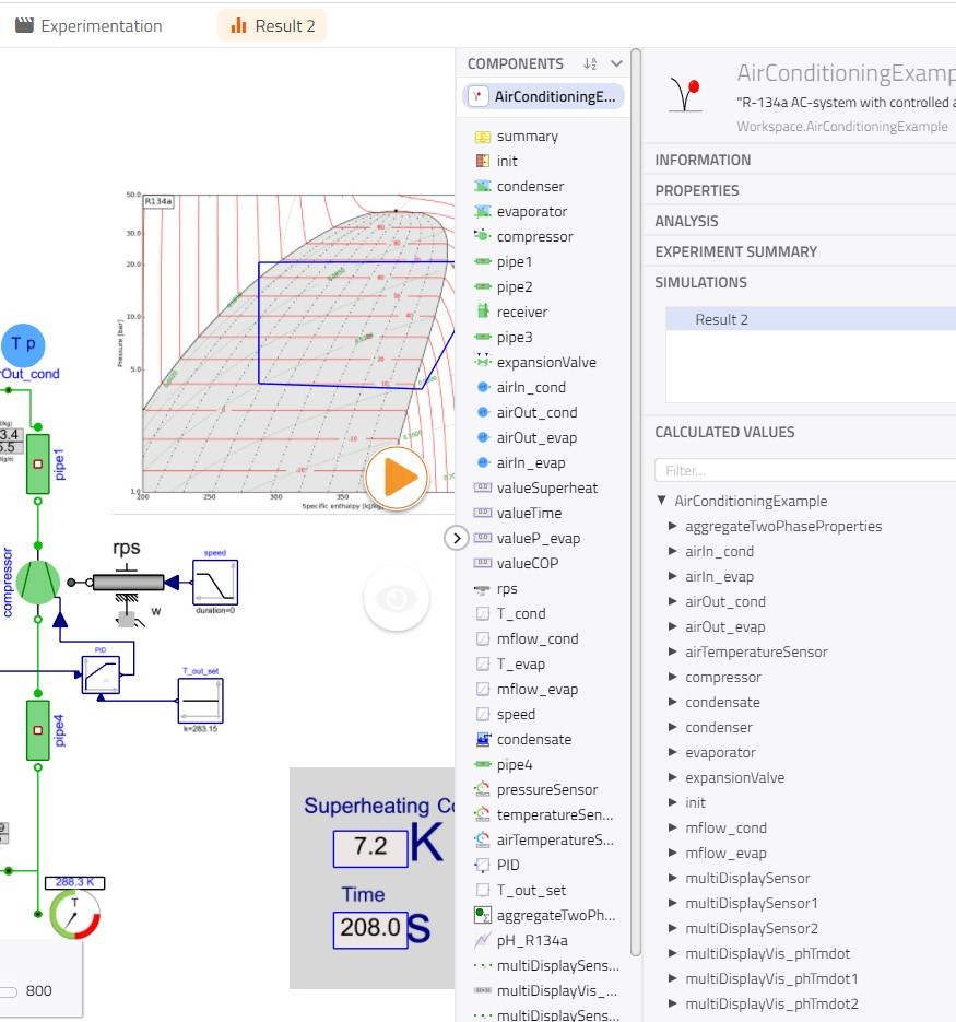
Result of using SBTL Media Creator in Modelon Impact
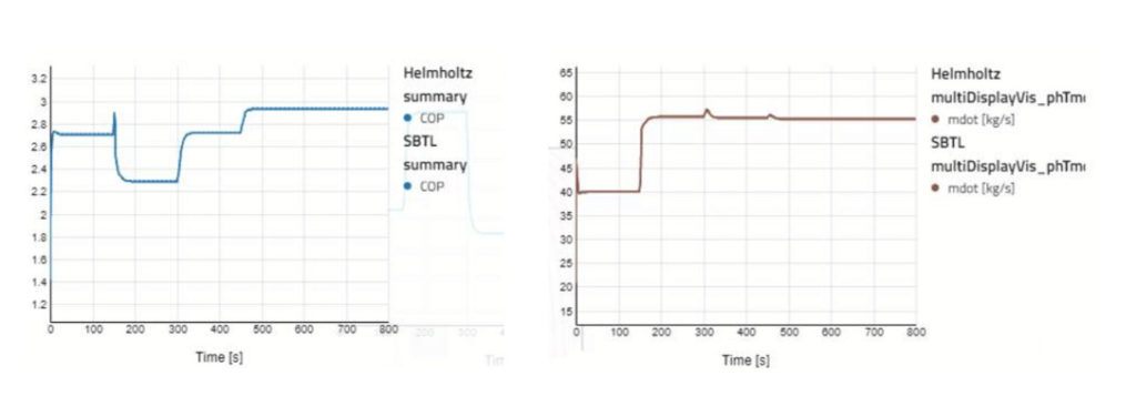
The example model above was 4 times faster to simulate (1 minute instead of 4 minutes) than the equivalent model using a Helmholtz equation based R134a medium implementation as the working fluid. The performance between the two cases is presented in Figure 6.