Mastering Modelica

My transition from Fortran procedural programming to acausal equation-based programming in Modelica
A bit more than a year ago I switched from procedural programming in Fortran to acausal (1) equation-based programming in Modelica. The transition to efficient usage of Dymola for model based design took about three weeks, including one week of training. To become a “Modelica hacker”, able to design completely new components and build well-structured libraries took another 1-2 months. Here’s my experience:
Phase 1: “Wow!” Your first contact with Modelica is amazing. It is possible to write equations as they are defined in the paper you use as a reference; you do not have to solve the equation system by extracting the derivatives, and you do not have to find and link a solver yourself. You see great potential in the combined graphical/text mode. You are really enthusiastic to get going.

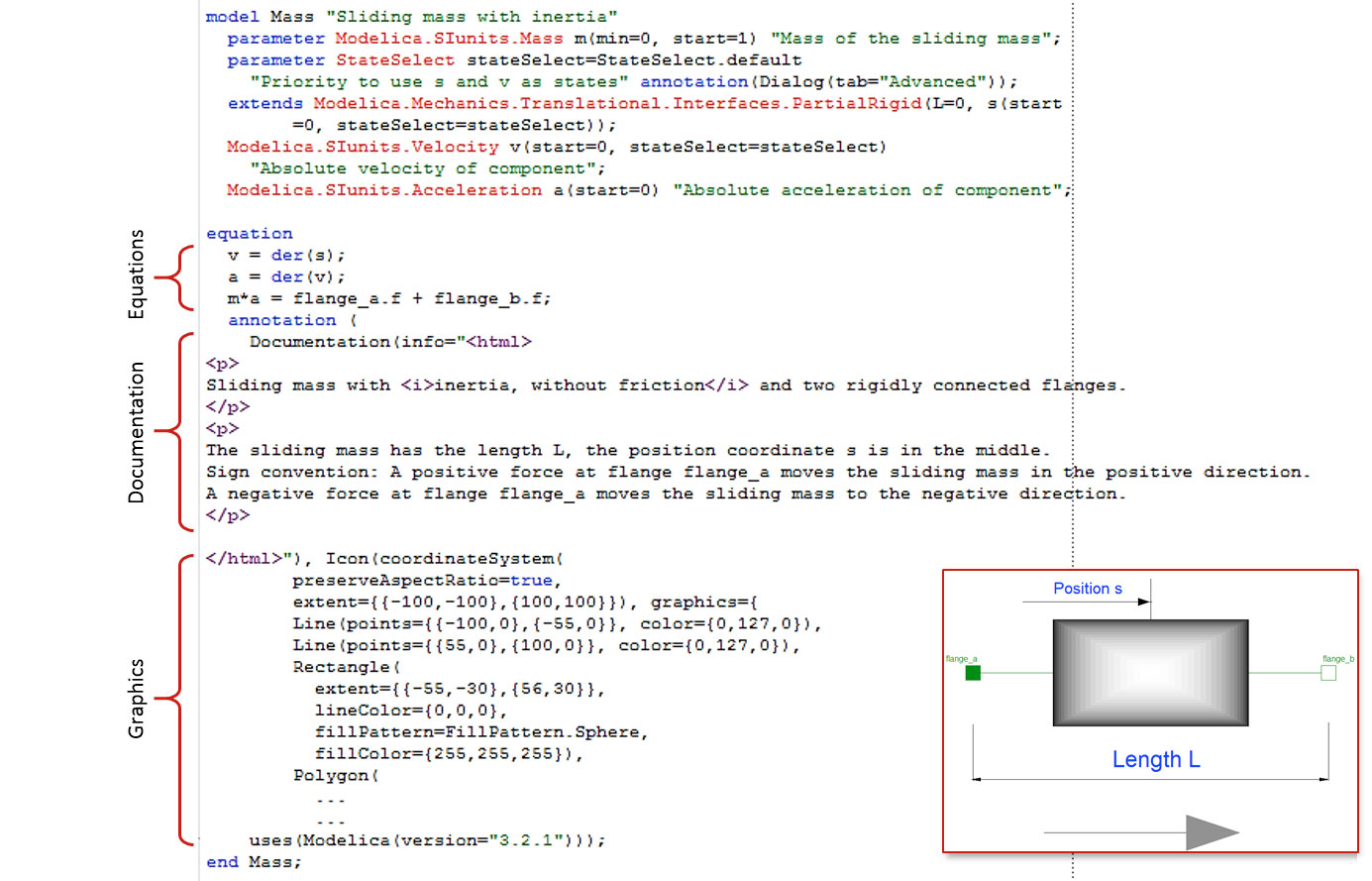
Modelica code (3) and graphical view for sliding mass in Modelica. Note the convenient way to define equations and the ‘der’ operator used for time derivatives. Also note that the documentation as well as graphical representation is a part of the Modelica code. The annotation is shortened for readability.
Phase 2: “Oh ***” When you start to use the language for real it is evident how vastly different it is from procedural programming. Everything is acausal, everything is written in equation form, and it is a bit difficult to get used to the very efficient but sometimes confusing object orientation. You realize how easy it is to make a mistake that returns a weird compilation error. The power of the language also makes it possible to do a lot of things wrong. I survived this phase thanks to the Modelica course I took. I strongly suggest that you take a course after 1-3 weeks of usage.
Phase 3: “Yes I can!” You start to build your first models. It works! Drag-and-drop functionality is awesome, and it is so easy to connect different domains and components with just a few clicks. This combined with direct access to the equations is great! You discover neat options like changing a model with two clicks, and duplication and extension of models. Now you’re becoming productive.

Usage of sliding mass model in Modelica (4). A system model is set up through drag-and -drop and visual connection of the components.
Phase 4: “Object-oriented hell! Where is the debugger???” You lose yourself in the very powerful but sometimes confusing advanced object-oriented library structures. To find the equation for a certain state is sometimes difficult. And, when you run the code and it stops, you realize it is not possible to debug like in Fortran or C code. You start to wonder how you are going to debug your code without a debugger. I survived this phase because I had great colleagues helping me out. I suggest that you have somebody either at your own company or at a support company help you through this phase.
Phase 5: “Nice, I can do this. For real. And it is very convenient.” You have understood how to debug (2), without a debugger. Advanced plotting and usage of logging options give you the possibility to quite easily find the cause of errors. You realize you never have to write a “print” statement, since all variables are automatically plotted. You never have to extract the derivatives of the ODE equation system or master numerical methods. You have to write very little code at all, since most components are available in various libraries. You have access to every equation in the program, but you can still represent almost everything graphically. You can mix various domains in seconds and build up complex systems using a simple drag-and-drop interface. The bottom line is: You can now concentrate on the engineering task. You are a Master of Modelica, with an extremely powerful simulation tool at your hands. Congratulations!

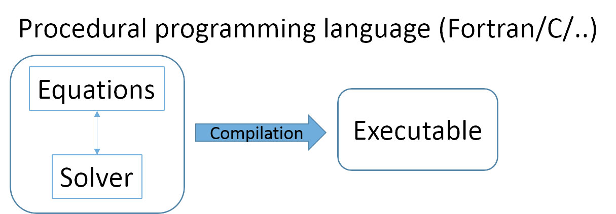
In procedural programming languages the equations are defined by declarations, and the solver is tightly connected to the code.

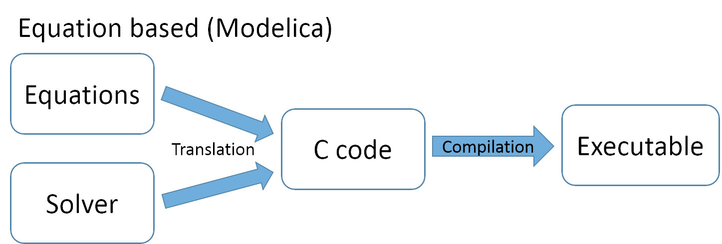
In equation based programming languages the equations are written as is, and the solver is bundled in translation.
Notes:
(1) – “Acausal modeling is a declarative modeling style, meaning modeling based on equations instead of assignment statements. Equations do not specify which variables are inputs and which are outputs, whereas in assignment statements variables on the left-hand side are always outputs (results) and variables on the right-hand side are always inputs.” Citation from section 2.7 in Principles of Object-oriented Modeling and Simulation with Modelica 2.1, Peter Fritzson, ISBN 978-0-471-47163-9
(2) – For further information on debugging, see e.g. Debugging Techniques for Equation-Based Languages, Dissertation by Peter Bunus, Linköping University, ISBN 91-7373-941-3 (2004)
(3) – Example from Modelica standard library; Modelica.Mechanics.Translational.Components.Mass
(4) – Example from Modelica standard library; Modelica.Mechanics.Translational.Examples.Oscillator